4 Bayesian Estimation to Nonlinear Regression Problem

Let $N(t)$ denotes the population size at time $t$. $N(t)$ is assumed to be a continuously differentiable function of $t$. Let the dynamics of the population is governed by the $\theta$-logistic growth equation \[\begin{equation}\label{eq:growth} \frac{\mathrm{d}N(t)}{\mathrm{d}t}=r_m N(t)\left[1-\left(\frac{N(t)}{K}\right)^{\theta}\right], ~ ~ ~ N(0)=N_0, \end{equation}\] where $r_m$ is the intrinsic growth rate of the population, $\theta$ is the curvature parameter depicting the shape of the per capita growth rate (PGR) and population density; $K$ is the carrying capacity of the environment. For $\theta=1$, we get the logistic growth function, which is a linearly decreasing function of $N$. For $\theta<1$ and $\theta>1$, the PGR-density relationship is concave upward and concave downward, respectively. The equation $\eqref{eq:growth}$ is a Bernoulli type differential equation whose solution is given by the following:

\[\begin{equation} N(t)= \frac{K}{\left\{1+ \left[\left(\frac{K}{N_0}\right)^{\theta}-1 \right]e^{-r_m t \theta}\right\}^{\frac{1}{\theta}} }. \end{equation}\]

It is easy to verify that as $t\to \infty$, $N(t) \to K$. In ecological literature, demographic and environmental variations are main source of stochastic population changes. If the population is subject to the environmental noise alone then the corresponding diffusion equation is described in the form of It$\hat{\mbox{o}}$ stochastic differential equation (SDE) as

\[\begin{equation} \mathrm{d}N(t)=rN(t)\left[1-\left(\frac{N(t)}{K}\right)^\theta\right]\mathrm{d}t + \sigma_eN(t)\mathrm{d}W(t). \end{equation}\]

If the dynamics of the population is subject to the demographic variation only, then the growth dynamics is governed by

\[\begin{equation}\label{eq:SDE} \mathrm{d}N(t) = rN(t)\left[1-\left(\frac{N(t)}{K}\right)^\theta\right]\mathrm{d}t+\sigma_d\sqrt{N(t)}\mathrm{d}W(t), \end{equation}\]

$\sigma^2_d$ and $\sigma^2_e$ are the demographic and environmental variances, respectively. $\{W(t), t\geq 0 \}$ is the standard Brownian motion, so that $\mathrm{d}W(t)\sim \mathcal{N}(0, \mathrm{d}t)$. We consider the population dynamics to be subjected to environmental stochasticity only. We seek to estimate the model parameters by using the maximum likelihood estimation method. To do that we first simulate the data following the above model using some assumed values of the parameters. The equation $\eqref{eq:SDE}$ can be described as follows,

\[\begin{equation} N(t+\Delta t) - N(t) = r N(t)\left[1-\left(\frac{N(t)}{K}\right)^\theta\right]\Delta t + \sigma_eN(t)\left[W(t + \Delta t) - W(t)\right]. \end{equation}\]

We have $\{t_0,t_1,\cdots,t_n\}$ be $n+1$ time points with $N(t_0) = X_0$, which is fixed. $W(t+\Delta t)- W(t)$ is the Brownian motion with mean $0$ and variance $\Delta t$. The simulation is carried out in the following way: The conditional distribution of $N(t +\Delta t)$ given $N(t)$ is given by a normal distribution with mean $N(t) + rN(t)\left[1-\left(\frac{N(t)}{K}\right)^\theta\right]\Delta t$ and variance $\sigma_e^2N(t)^2\Delta t$ and notionally can be written as follows:

\[\begin{equation} N(t + \Delta t) -N(t)|N(t) \sim \mathcal{N}\left(rN(t)\left[1- \left(\frac{N(t)}{K}\right)^{\theta}\right]\Delta t, \sigma_e^2 N(t)^2 \Delta t\right). \end{equation}\]

We fixed $t_0 = 0$ and $\Delta t =0.1$. Let $N_{t_0},N_{t_1},\dots,N_{t_n}$ are the $n+1$ population sizes are generated using the above rule. The likelihood function $\mathcal{L}(\boldsymbol{\beta})$ of the sample $N_0$, $N_1$, $N_2$, $\cdots$, $N_n$ is the joint density of the observations treated as a function of the parameter $\boldsymbol{\beta}$. The method of maximum likelihood provides as estimate of $\boldsymbol{\beta}$ any value $\hat{\boldsymbol{\beta}}$ which maximizes $\mathcal{L}$. Note that $\{N_{t_i}\}_{i=0}^{n}$ are not independent but the differences are assumed to be independent, So the likelihood function can be written as

\[\begin{eqnarray*} \mathcal{L} &=& f\left(N_1,N_2,\dots,N_n|N_0; r,K,\theta,\sigma_e\right)\\ &=& f\left(N_1,N_2,\dots,N_n|N_0;\boldsymbol{\beta}\right)\\ &=& f\left(N_n|N_{n-1},\dots,N_0;\boldsymbol{\beta}\right)f\left(N_{n-1}|N_{n-2},\dots,N_0;\tilde{\beta}\right)\dots f\left(N_1|N_0;\tilde{\beta}\right)\\ &=&\prod_{i=1}^{n} f\left(N_i|N_{i-1}\dots,N_0;\boldsymbol{\beta}\right)\\ &=& \prod_{i=1}^{n}f\left(N_i|N_{i-1};\beta\right)\\ &=& \prod_{i=1}^{n}\frac{1}{\sqrt{2\pi} \sigma_eN_{i-1} {\sqrt{\Delta t_i}}}e^{-\frac{1}{2\sigma^2_e}\Sigma_{i=1}^{n}\left(\frac{N_i-\mu_{N_{i-1}}}{N_{i-1}}\right)^2}\\ &=& \frac{1}{\sqrt{2\pi}^n(\sigma_e)^n(\prod_{i=1}^{n}N_{i-1} {\sqrt{\Delta t_i}})}e^{-\frac{1}{2\sigma^2_e}\Sigma_{i=1}^{n}\left(\frac{N_i-\mu_{N_{i-1}}}{N_{i-1}}\right)^2} \end{eqnarray*}\]

where $\mu_{N_i} =N(t_i) + r N(t_i)\left[1-\left(\frac{N(t_i)}{K}\right)^\theta\right]\Delta t$. The log-likelihood function is given by

\[\begin{eqnarray} l(\beta)&=&\log \mathcal{L}(\beta)\\ &=& -n\ln \sqrt{2\pi}-n\ln \sigma_e-\ln \prod_{i=1}^{n}(N_{i-1}\sqrt{\Delta t_i})-\frac{1}{2 \sigma^2_e}\sum_{i=1}^{n}\left(\frac{N_i - \mu_{N_{i-1}}}{N_{i-1}}\right)^2\\ &=& -n \ln (\sqrt{2\pi})- n \ln \sigma_e- \sum_{i=1}^{n}\ln \sqrt{\Delta t_i}-\sum_{i=1}^{n}\ln (N_{i-1})-\frac{1}{2\sigma^2_e}\sum_{i=1}^{n}\left[\frac{N_i-N_{i-1}-r N_{i-1}\left[1-\left(\frac{N_{i-1}}{K}\right)^\theta\right]\Delta t_i}{N_{i-1}}\right]^2 \end{eqnarray}\]

4.1 Estimation of Parameters

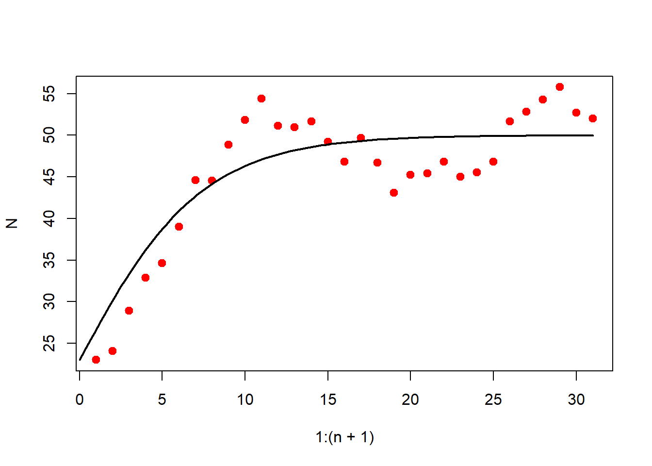
Consider $\{ N_1,N_2,\cdots,N_{n+1}\}$ be the observed time series data. The absolute change in population size at time $t$ is approximated as \[\frac{\mathrm{d}N(t)}{\mathrm{d}t} \approx \frac{N(t+\Delta t)-N(t)}{\Delta t}.\] We assume the yearly changes in population size, so that $\Delta t=1$. The relative changes in population sizes is given by

\[\begin{equation} R(t) = \frac{1}{N}\frac{\mathrm{d}N(t)}{\mathrm{d}t} = \frac{\mathrm{d}}{\mathrm{d}t} \log N \approx \log N(t+1)- \log N(t). \end{equation}\]

So, for a given population time series data of size $n+1$, we have $n$ many observed per capita growth rates $\{R(1),R(2),\cdots,R(n)\}$. We would like to investigate the dynamics of the population when it is subject to environmental stochastic perturbations alone. The following stochastic differential equation has been used to describe to population changes that is exposed to environmental variability.

\[\begin{equation}\label{eq:theta logistic} \mathrm{d}N = r_m N(t) \left[ 1-\left( \frac{N(t)}{K}\right)^{\theta} \right]\mathrm{d}t + \sigma_{e} N(t)\mathrm{d}W(t) , \end{equation}\]

where $\sigma_{e}$ represents the intensity of the stochastic perturbation and $W(t)$ is the one dimensional Brownian motion which satisfies $\mathrm{d}W(t) \approx W(t+\mathrm{d}t)-W(t) \sim \mathcal{N}(0,\mathrm{d}t)$. Our goal is to estimate the parameters of the stochastic model by employing Bayesian statistical methods. First we compute the likelihood function of the model parameters given the population size. It is to be noted that the likelihood function can be written either by conditional on the population size $\{N_t\}$ or on the growth rates $\{R_t\}$. We can use the either observations on $\{R_t\}$ or $\{N_t\}$ to obtain the posterior distribution of the model parameters. Now, we shall write down the likelihood function given the population time series. Using the equation $\eqref{eq:theta logistic}$ and utilizing the distributional assumptions, we see that the absolute changes in the population size, conditional on the current size, is normally distributed. So we obtain the following (assuming $\Delta t =1$):

\[\begin{align} N(t+1)-N(t)|N(t) &\sim \mathcal{N}\left(r_m N(t) \left[ 1-\left( \frac{N(t)}{K}\right)^{\theta} \right], \sigma_{e}^2 N(t)^2 \right) \notag \\ \frac{N(t+1)-N(t)}{N(t)}| N(t) &\sim \mathcal{N}\left(r_m \left[ 1-\left( \frac{N(t)}{K}\right)^{\theta} \right], \sigma_{e}^2 \right) \notag \\ N(i+1)-N(i) &\sim \mathcal{N}\left(r_m N(i)\left[1-\left( \frac{N(i)}{K}\right)^{\theta} \right], \sigma_{e}^2 N(i)^2 \right) \notag \\ N(i+1)|N(i) &\sim \mathcal{N}\left(N(i) + r_m N(i)\left[1-\left( \frac{N(i)}{K}\right)^{\theta} \right], \sigma_{e}^2 N(i)^2 \right) \label{eq:N_i} \end{align}\]

We can estimate the parameters using ($\ref{eq:N_i}$) using the method of maximum likelihood. Therefore by using ($\ref{eq:N_i}$), our goal is to estimate parameters $r_m$, $\theta$, $K$, $\sigma_e^2$. If we use $R_t$ values, then the following equation will be used for computation of the likelihood.

\[\begin{equation} R(t)|N(t) \sim \mathcal{N}\left(r_m\left[1-\left( \frac{N(t)}{K}\right)^{\theta} \right],\sigma_{e} ^2\right) \label{eq:R_T}, \end{equation}\] so that the log-likelihood function will be,

\[\begin{equation}\label{eq:likelihood} \mbox{likelihood} = -\frac{n}{2}\log(2\pi)-\frac{n}{2}\log(\sigma_e^2)-\frac{1}{2\sigma_e^2}\sum_{i=1}^{n}\left\lbrace R(i)- r_m\left[1-\left( \frac{N(i)}{K}\right)^{\theta}\right] \right\rbrace^2 . \end{equation}\]

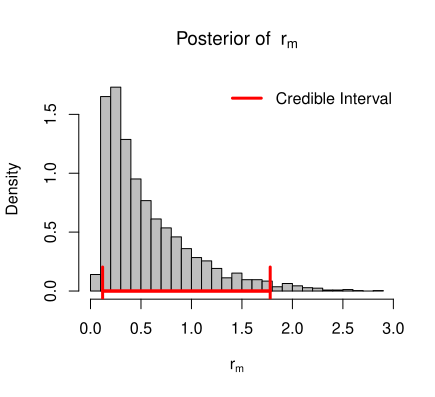
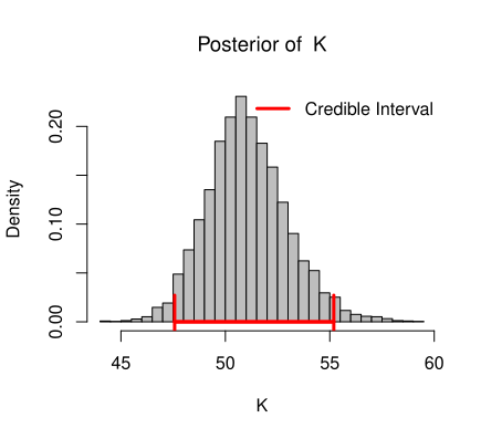
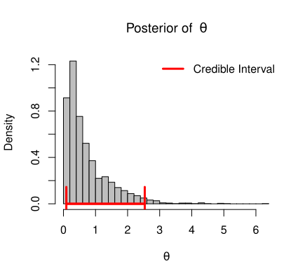
To draw inference about $r_m$, $\theta$, $K$ and $\sigma_e^2$, we consider inverted gamma prior for variance term $\sigma_e^2$, gamma prior for $\theta$, normal prior for $K$ and normal prior for $r_m$. Then the complete Bayesian model for this data can be written as,

\[\begin{align*} N(i+1)|N(i),r_m,\theta,K,\sigma_e^2 &\sim \mathcal{N}\left(N(i) + r_m N(i)\left[1-\left( \frac{N(i)}{K}\right)^{\theta} \right], \sigma_{e}^2 N(i)^2 \right) \\ r_m|\alpha_0,\beta_0 &\sim \mathcal{N}(\alpha_0,\beta_0)\\ K| \mu_K,\sigma_K^2 &\sim \mathcal{N}(\mu_K,\sigma_K^2)\\ \theta|\alpha_1,\beta_1 &\sim \mathcal{G}(\alpha_1,\beta_1) \\ \sigma_e^2|\alpha_2,\beta_2 &\sim \mathcal{IG}(\alpha_2,\beta_2), \end{align*}\]

where $\alpha_0,\alpha_1,\alpha_2,\beta_0,\beta_1,\beta_2,\mu_K$, and $\sigma_K^2$ are hyper-parameters and assumed to be known. As the starting population size is known, $P(N(1)=N_0)=1$. We take $N(1)=N_0$ as the starting population size and assumed to be a fixed quantity. The joint posterior distribution of $r_m,\theta,K,\sigma_e^2$ can be written as,

\[\begin{equation*} f(r_m,\theta,K,\sigma_e ^2|\boldsymbol{N})=\frac{f(\boldsymbol{N},r_m,\theta,K,\sigma_e ^2)}{f_{\boldsymbol{N}}(\boldsymbol{N})}, \end{equation*}\] where $\boldsymbol{N}=(N(1),N(2),\cdots,N(n+1))'$ represents the data and $f_{\boldsymbol{N}}(\boldsymbol{N})$ is the marginal distribution of $\boldsymbol{N}$.

\[\begin{equation}\label{eq:27} f\left(r_m,\theta,K,\sigma_e^2|\boldsymbol{N}\right) = \frac{f\left(\boldsymbol{N}|r_m,\theta,K,\sigma_e^2\right)\cdot f\left(r_m,\theta,K,\sigma_e^2\right)}{f(\boldsymbol{N})}. \end{equation}\] We assume that $r_m,\theta,K,\sigma_e^2$ are independent variables, therefore $f(r_m,\theta,K,\sigma_e ^2)$ can be written as,

\[\begin{equation} f\left(r_m,\theta,K,\sigma_e^2\right)=f(r_m)\cdot f(\theta) \cdot f(K) \cdot f\left(\sigma_e^2\right). \end{equation}\] So, equation ($\ref{eq:27}$) becomes, \[\begin{eqnarray*} f\left(r_m,\theta,K,\sigma_e^2|\boldsymbol{N}\right) &\propto& f\left(\boldsymbol{N}|r_m,\theta,K,\sigma_e^2\right)\cdot f\left(r_m,\theta,K,\sigma_e^2\right) \\ &\propto& f(\boldsymbol{N}|r_m,\theta,K,\sigma_e ^2)\cdot f(r_m)\cdot f(\theta) \cdot f(K) \cdot f(\sigma_e ^2)~~[\mbox{independence of priors}] \\ &\propto& \left[\prod_{i=1}^{n} f\left(N(i+1)|N(i)\right)\right]\cdot f(r_m)\cdot f(\theta) \cdot f(K) \cdot f(\sigma_e ^2). \end{eqnarray*}\]

The right hand side of the above expression is product of the likelihood and the prior, which is nothing but unnormalized joint posterior distribution of parameters. Since, the distribution does not follow some common known distribution, we use the Gibbs sampling method that simulates samples from the conditional distribution. So we generate random sample from conditional posterior distribution of each parameters. However, it is observed that in this case also the conditional posterior does not follow any known distribution. So, we use grid approximation algorithm to approximate the posterior probability distribution.

Let $\boldsymbol{\beta} = \left(r_m,\theta, K, \sigma_e^2\right)$. Since, $N(i)$’s are not independent, so the likelihood can be written as,

\[\begin{eqnarray*} \mbox{likelihood} &=& f\left(N(1),N(2),\cdots , N(n+1) ; \beta \right) \\ &=& f\left(N(n+1)|N(n) ; \beta \right)\cdot f\left(N(n)|N(n-1) ; \beta \right) \cdots f\left(N(2)|N(1) ; \beta \right)\cdot f\left(N(1) ; \beta \right) \\ &=& \prod_{i=1}^{n} f\left(N(i+1)|N(i) ; \beta \right)\cdot f\left(N(1); \beta \right). \end{eqnarray*}\]

We assume that the initial population size to be known so that $f\left(N(1);\beta \right) = 1$.

\[\begin{eqnarray*} \mbox{likelihood} &=& \prod_{i=1}^{n} f\left(N(i+1)|N(i) ; \beta \right) \\ &=& \prod_{i=1}^{n}\left[\frac{1}{\sqrt[]{2\pi}\sigma_e^2 N(i)} e^{-\frac{\left\lbrace N(i+1)-N(i)- r_m N(i)\left[1-\left( \frac{N(i)}{K}\right)^{\theta} \right]\right\rbrace^2} {2\sigma_e^2 N(i)^2}}\right]\\ &=&\prod_{i=1}^{n} \left[\frac{1}{\sqrt[]{2\pi}\sigma_e^2 N(i)} e^{{-\frac{1}{2\sigma_e^2}\left\lbrace \frac{N(i+1)-N(i)}{N(i)}-r_m\left[1-\left( \frac{N(i)}{K}\right)^{\theta}\right] \right\rbrace}^{\theta} }\right]\\ &=& \frac{1}{(\sqrt[]{2\pi})^n}\frac{1}{(\sigma_e)^n}\frac{1}{\prod_{i=1}^{n} N(i)} e^{-\frac{1}{2\sigma_e^2}\sum_{i=1}^{n}\left\lbrace R(i)- r_m\left[1-\left( \frac{N(i)}{K}\right)^{\theta}\right] \right\rbrace^2}. \end{eqnarray*}\]

The log-likelihood can be given as,

\[\begin{equation} \mbox{log-likelihood} = -\frac{n}{2}\log(2\pi)-\frac{n}{2}\log(\sigma_e^2)-\sum_{i=1}^{n}\log(N(i))-\frac{1}{2\sigma_e^2}\sum_{i=1}^{n}\left\lbrace R(i)- r_m\left[1-\left( \frac{N(i)}{K}\right)^{\theta}\right] \right\rbrace^2. \end{equation}\]

To compute the conditional posterior following process has been carried out,

\[\begin{eqnarray*} f(r_m|\theta,K,\sigma_e^2,\boldsymbol{N})&=&\frac{f(\boldsymbol{N},r_m,\theta,K,\sigma_e^2)}{f(\theta,K,\sigma_e^2,\boldsymbol{N})}\\ &=& \frac{f(\boldsymbol{N}|r_m,\theta,K,\sigma_e^2)\cdot f(r_m,\theta,K,\sigma_e^2)}{f(\boldsymbol{N},\theta,K,\sigma_e^2)}\\ &=&\frac{f(\boldsymbol{N}|r_m,\theta,K,\sigma_e^2)\cdot\pi(r_m)\pi(\theta)\pi(K)\pi(\sigma_e^2)}{f(\boldsymbol{N}|\theta,K,\sigma_e^2)\cdot f(\theta,K,\sigma_e^2)}\\ &=&\frac{f(\boldsymbol{N}|r_m,\theta,K,\sigma_e^2)\cdot \pi(r_m)\cdot \pi(\theta)\cdot \pi(K)\cdot\pi(\sigma_e^2)}{f(\boldsymbol{N}|\theta,K,\sigma_e^2)\cdot \pi(\theta)\cdot \pi(K)\cdot\pi(\sigma_e^2)}\\ &=&\frac{f(\boldsymbol{N}|r_m,\theta,K,\sigma_e^2)\cdot \pi(r_m)}{f(\boldsymbol{N}|\theta,K,\sigma_e^2)}. \end{eqnarray*}\] Let $m=f(\boldsymbol{N}|\theta,K,\sigma_e^2)$, be the joint marginal probability density function of the data. \[\begin{eqnarray} f(r_m|\theta,K,\sigma_e^2,\boldsymbol{N}) &\propto& f(\boldsymbol{N}|r_m,\theta,K,\sigma_e^2)\cdot \pi(r_m) \notag\\ &\propto& \prod_{i=1}^{n} f(N_{i+1}|N_i ; r_m,\theta,K,\sigma_e^2)\cdot \pi(r_m). \end{eqnarray}\] Similarly,

\[\begin{eqnarray} f(\theta|r_m,K,\sigma_e^2,\boldsymbol{N})&\propto& \prod_{i=1}^{n} f(N_{i+1}|N_i ; r_m,\theta,K,\sigma_e^2)\cdot \pi(\theta)\\ f(K|r_m,\theta,\sigma_e^2,\boldsymbol{N})&\propto& \prod_{i=1}^{n} f(N_{i+1}|N_i ; r_m,\theta,K,\sigma_e^2)\cdot \pi(K)\\ f(\sigma_e^2|r_m,\theta,K,\boldsymbol{N}) &\propto& \prod_{i=1}^{n} f(N_{i+1}|N_i ; r_m,\theta,K,\sigma_e^2)\cdot \pi(\sigma_e^2). \end{eqnarray}\]

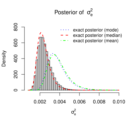
In Bayesian linear regression we already verify that the variance (specially $\phi$) after observed data follows $\mathcal{IG}\left( \mbox{shape} = \alpha+\frac{n}{2}, \mbox{rate} =\frac{1}{2} \sum_{i=1}^{n}\left(y_i-\beta_0-\beta_1x_i\right)^2 + \gamma\right)$. Similarly here we expect posterior distribution of variance($\sigma_e^2$) as follows:

\[\begin{equation}\label{eq:post_sigma_sq} \sigma_e^2|\boldsymbol{N} \sim \mathcal{IG}\left( \mbox{shape} = \alpha_2 +\frac{n}{2}, \mbox{rate} =\frac{1}{2}\sum_{i=1}^{n}\left(y_i- r_m \left\lbrace 1-\left( \frac{N(t)}{K}\right)^{\theta} \right\rbrace\right)^2+\beta_2\right). \end{equation}\]

Note

If the prior distribution $\pi(r_m)$ is considered to be $\mbox{gammma}(\alpha, \beta)$ which takes only positive values, then task of estimation of a declining population may be underestimated.

Note

To reduce the computational time a correct choice of priors is required. In this case, since $K$ is a property of the environment, it should not change drastically. Posterior sample of k should not vary too much away from the prior mean of $K$.

Note

If the prior distribution $\pi(r_m)$ is considered to be $\text{gamma}(\alpha, \beta)$ which takes only positive values, then the task of estimation of a declining population may be underestimated.

Note

To reduce the computational time, a correct choice of priors is required. In this case, since $K$ is a property of the environment, it should not change drastically. The posterior sample of $K$ should not vary too much from the prior mean of $K$.

The above structure of the posterior density function of $\sigma_e^2$ given in the equation $\eqref{eq:post_sigma_sq}$ is verified by the simulation for the simulated data.

4.2 Simulation study

4.2.1 Data Generation

Time series data of population size is generated using $r_m=0.5,~~ \theta=0.5,~~K=50,~~\sigma_e^2=0.0025$. The initial population size is set as $N_0 = 23$ and the length of the simulated series is $n=30$. The full Bayesian model is described as follows:

\[\begin{align} R(t)|N(t) &\sim \mathcal{N}\left(r_m\left[1-\left( \frac{N(t)}{K}\right)^{\theta} \right],\sigma_{e} ^2\right)\label{eq:logistic model} \\ r_m|\alpha_0,\beta_0 &\sim \mathcal{N}(\alpha_0,\beta_0)\notag\\ K| \mu_K,\sigma_K^2 &\sim \mathcal{N}(\mu_K,\sigma_K^2)\notag\\ \theta|\alpha_1,\beta_1 &\sim \mathcal{G}(\alpha_1,\beta_1)\notag\\ \sigma_e^2|\alpha_2,\beta_2 &\sim \mathcal{IG}(\alpha_2,\beta_2).\notag \end{align}\]

# parameters values for simulating the data
rm = 0.5 # intrinsic growth rate
theta = 0.5 # parameter for strength of density dependence
K = 50 # carrying capacity of the environment
sig_2e = 0.0025 # variance of the environmental perturbation
n = 30 # length of the time series = n+1
N1 = 23 # initial population size

set.seed(471)
N = numeric(n + 1) # storage the simulated time series
N[1] = N1 # initial population size.
for(i in 1:(length(N)-1)){
  r = rnorm(n =1, mean = rm*(1-(N[i]/K)^theta), sd = sqrt(sig_2e)) #   simulating growth rate
  N[i+1] = N[i]*exp(r) # simulate next generation
}
#print(N) # printing population size
plot(1:(n+1), N, type= "p", lwd=2, col = "red", pch = 19)

fun_logistic = function(x){ # Deterministic solution of the generalized logistic equation
K/(1+((K/N1)^theta-1 )*exp(-rm*x*theta) )^(1/theta)
}
curve(fun_logistic, 0, n+1, add= TRUE, lwd=2)

Figure 4.1: Plot of simulated data for the study of Nonlinear regression generated using the model given in the equation ($\ref{eq:logistic model}$). The parameters values are fixed as $r_m=0.5, \theta=0.5, K=50, \sigma_e^2=0.0025$, and initial population size taken as $N_0=23$, generated data of length $n=30$.

4.2.2 Define Prior distributions

For generated time series, we want to generate values from posterior of each parameter$(r_m,K,\theta,\sigma_e^2)$. For simulation purpose, we first define the prior functions for the prior distribution given in the equation ($\ref{eq:logistic model}$) by considering the values of hyper-parameters as $\beta_0=1, \sigma_K^2=3, \alpha_1=1, \beta_1=1, \alpha_2=1, \beta_2= 0.0001$. Prior mean of $K$ and $r_m$ that is $\mu_K$ and $\alpha_0$ are obtained by fitting the logistic growth equation using nonlinear least squares method ($\texttt{nls}$, in $\texttt{R}$). The package $\texttt{invgamma}$ (Kahle and Stamey 2017) has been used for generating random numbers from the inverted gamma distribution.

prior_mean_rm = coef(fit)[1]
prior_sd_rm = 1
fun_prior_rm = function(x){ # Prior specification for r_m
  dnorm(x, prior_mean_rm, prior_sd_rm)
}

prior_mean_K = coef(fit)[2]
prior_sd_K = 3
fun_prior_K = function(x){ # Prior specification for K
  dnorm(x, prior_mean_K, prior_sd_K)
}

alpha_1 = 1
beta_1 = 1
fun_prior_theta = function(x){ # Prior specification for theta
  dgamma(x, shape = alpha_1, rate = beta_1)
}

library(invgamma)
alpha_2 = 1
beta_2 = 0.0001
fun_prior_sig_2e = function(x){ # Prior specification for inverted gama
  dinvgamma(x, shape = alpha_2, rate = beta_2)
}

As mentioned in the Section 4.1, the exact form of the conditional posterior distribution is not known, so grid approximation has been utilized to approximate the conditional posterior density function. In the following code, we have created grid within an interval specified for each parameter. This initial choice is important as this act as a support for the density function. Finer the grid is more accurate is the posterior approximation.

# Specification of grid values for approximating the posterior
step = 0.01
grid_rm = seq(from = -3, to =3, by = step)
grid_K = seq(from = 40, to = 60, by = step)
grid_theta = seq(from = 0, to =10, by = step)
grid_sig_2e = seq(from = 0.0001 , to =0.01, by = 0.00001)

4.2.3 Likelihood function

In the following code we define the likelihood function. Note that we have directly computed the log-likelihood values to avoid truncation error.

likelihood = function(data, param){
  rm = param[1]
  K = param[2]
  theta = param[3]
  sig_2e = param[4]

  x = data[,1] # population size
  y = data[,2] # per capita growth rates

  log_lik = -n*log(sqrt(2*pi)) - (n/2)*log(sig_2e) - sum(((y-rm*(1-(x/K)^theta))^2/(2*sig_2e)))
  return(exp(log_lik))
}

4.2.4 Calculation of Posterior distribution

First of all we have set 100000 as a number Markov Chain samples to be generated. Then we have fixed the initial values of the parameters and defined the arrays for storing the posterior values of the parameters in $\texttt{R}$ as follows:

iter = 100000 # Length of the chain to be simulated
post_rm = rep(NA, iter) # posterior values of r_m
post_K = rep(NA, iter) # posterior values of K
post_theta = rep(NA, iter) # posterior values of theta
post_sig_2e = rep(NA, iter) # posterior values of simga_2e

param = c(0.2, 40, 1, 0.02) # starting of the chain

# initialization of the chain
post_rm[1] = param[1]
post_K[1] = param[2]
post_theta[1] = param[3]
post_sig_2e[1] = param[4]

Next we carried out the Gibbs sampling and grid approximation of the posterior distribution. At each Gibbs sampling step (outer loop), the conditional posterior has been approximated by grid approximation (four inner loop for four parameters).

for(i in 2:iter){ # loop for iteration of Gibbs sampling
  # section for rm
  tmp_post_rm = numeric(length = length(grid_rm))
  for(j in 1:length(grid_rm)){
      param = c(grid_rm[j], post_K[i-1], post_theta[i-1], post_sig_2e[i-1])
      tmp_post_rm[j] = likelihood(data = data, param = param)*fun_prior_rm(grid_rm[j])
    }
  prob = tmp_post_rm/sum(tmp_post_rm)
  post_rm[i] = sample(grid_rm, size = 1, prob = prob)

  # section for K
  tmp_post_K = numeric(length = length(grid_K))
  for(j in 1:length(grid_K)){
    param = c(post_rm[i], grid_K[j], post_theta[i-1], post_sig_2e[i-1])
    tmp_post_K[j] = likelihood(data = data, param = param)*fun_prior_K(grid_K[j])
    }
  prob = tmp_post_K/sum(tmp_post_K)
  post_K[i] = sample(grid_K, size = 1, prob = prob)

  # section for theta
  tmp_post_theta = numeric(length = length(grid_theta))
  for(j in 1:length(grid_theta)){
    param = c(post_rm[i], post_K[i], grid_theta[j], post_sig_2e[i-1])
    tmp_post_theta[j] = likelihood(data = data, param = param)*fun_prior_theta(grid_theta[j])
    }
  prob = tmp_post_theta/sum(tmp_post_theta)

  post_theta[i] = sample(grid_theta, size = 1, prob = prob)

  # section for sig_2e
  tmp_post_sig_2e = numeric(length = length(grid_sig_2e))
  for(j in 1:length(grid_sig_2e)){
    param = c(post_rm[i], post_K[i], post_theta[i], grid_sig_2e[j])
    tmp_post_sig_2e[j] = likelihood(data = data, param = param)*fun_prior_sig_2e(grid_sig_2e[j])
    }
  prob = tmp_post_sig_2e/sum(tmp_post_sig_2e)
  post_sig_2e[i] = sample(grid_sig_2e, size = 1, prob = prob)

} # loop ends for Gibbs iteration

By executing the above code, we have obtained the 1,00,000 sample values from the posterior density of $r_m, K, \theta$, and $\sigma_e^2$. We stored them in the local directory on system for the further analysis.

post_param_vals = data.frame(post_rm,post_K,post_theta,post_sig_2e)
setwd("specify path here")
filename = paste0("output",seed, ".txt")
write.table(post_param_vals, file = filename, col.names = TRUE)

Trace plot is a key diagnostic tool used in Bayesian statistics to assess the behavior and convergence of MCMC chains. So we have plotted the traceplot of posterior values obtained using Grid and Gibbs approximation using following code:

filename = paste0("output",seed, ".txt")
post_vals = read.table(file = filename, header = TRUE)

#traceplot
par(mfrow=c(2,2))
plot(post_vals$post_rm, type = "l", main = bquote("Trace plot of"~ r[m]),col = "red")
plot(post_vals$post_K, type = "l", main = bquote("Trace plot of"~ K),col = "red")
plot(post_vals$post_theta, type = "l", main = bquote("Trace plot of"~ theta),col = "red")
plot(post_vals$post_sig_2e, type = "l", main = bquote("Trace plot of"~ sigma[e]^2),col = "red")

We have kept initial half i.e 50,000 sample values as a burn-in period for each parameter. After the burn-in period from remaining 50,000 sample posterior values, using appropriate step for thinning (using auto-correlation function, $) we have reduced the autocorrelation between the successive samples to get reliable estimate of parameters. Next we have plot the histogram of posterior distribution of all parameters using following code and depicted in the Figure 4.2.

cut = 0.5 # burn-in chain (first 50,000 values as burn-in period)

# for rm
u = post_vals$post_rm[ceiling(iter*cut):iter] # after burn in period
index = seq(1,length(u), by = 20) # thining
post_rm_thinning = u[index] # values after thinning
acf(post_rm_thinning,main = bquote("acf of posterior "~rm)) # autocorrelation
post_interval_rm = quantile(post_rm_thinning, c(2.5, 97.5)/100) #credible interval for rm
hist(post_rm_thinning, probability = TRUE,main = bquote("Posterior of "~ r[m]),
xlab = expression(r[m]),col = "grey", breaks = 40)
arrows(post_interval_rm[1], 0, post_interval_rm[2], 0, lwd=3, angle = 90,col = "red", code = 1)
arrows(post_interval_rm[2], 0, post_interval_rm[1], 0, lwd=3, angle = 90,col = "red", code = 1)
legend("topright",legend = c("Credible Interval"),lwd = 3, col = "red",lty = 1,cex = 1, bty = "n")

# for K
u = post_vals$post_K[ceiling(iter*cut):iter] # after burn in period
index = seq(1,length(u), by = 10) # thining
post_K_thinning = u[index] # values after thinning
acf(post_K_thinning,main = bquote("acf of posterior "~K)) # autocorrelation
post_interval_K = quantile(post_K_thinning, c(2.5, 97.5)/100) #credible interval for K
hist(post_K_thinning, probability = TRUE,main = bquote("Posterior of "~ K),
xlab = expression(K),col = "grey", breaks = 40)
arrows(post_interval_K[1], 0, post_interval_K[2], 0, lwd=3, angle = 90, col = "red", code = 1)
arrows(post_interval_K[2], 0, post_interval_K[1], 0, lwd=3, angle = 90, col = "red", code = 1)
legend("topright",legend = c("Credible Interval"),lwd = 3, col = "red",lty = 1,cex = 1, bty = "n")

# for theta
u = post_vals$post_theta[ceiling(iter*cut):iter] # after burn in period
index = seq(1,length(u), by = 20) # thining
post_theta_thinning = u[index] # values after thinning
acf(post_theta_thinning,main = bquote("acf of posterior "~theta)) # autocorrelation
post_interval_theta = quantile(post_theta_thinning, c(2.5, 97.5)/100) #credible interval for theta
hist(post_theta_thinning, probability = TRUE,main = bquote("Posterior of "~ theta),xlab = expression(theta),col = "grey", breaks = 40)
arrows(post_interval_theta[1], 0, post_interval_theta[2], 0, lwd=3, angle = 90, col = "red", code = 1)
arrows(post_interval_theta[2], 0, post_interval_theta[1], 0, lwd=3, angle = 90, col = "red", code = 1)
legend("topright",legend = c("Credible Interval"),lwd = 3, col = "red",lty = 1,cex = 1, bty = "n")

# for sigma_e^2
u = post_vals$post_sig_2e[ceiling(iter*cut):iter] # after burn in period
index = seq(1,length(u), by = 1) # thining
post_sig_2e_thinning = u[index] # values after thinning
acf(post_sig_2e_thinning,main = bquote("acf of posterior "~sigma[e]^2))
post_interval_sig_2e = quantile(post_sig_2e_thinning, c(2.5, 97.5)/100)
#credible interval for sig_2e
hist(post_sig_2e_thinning, probability = TRUE,main = bquote("Posterior of "~ sigma[e]^2),xlab = expression(sigma[e]^2),col = "grey", breaks = 40, ylim = c(0,800))
arrows(post_interval_sig_2e[1], 0, post_interval_sig_2e[2], 0, lwd=3, angle = 90, col = "red", code = 1)
arrows(post_interval_sig_2e[2], 0, post_interval_sig_2e[1], 0, lwd=3, angle = 90, col = "red", code = 1)
legend("topright",legend = c("Credible Interval"),lwd = 3, col = "red",lty = 1,cex = 1, bty = "n")

For $\sigma_e^2$, due to conjugacy the posterior density is predictable, but good approximation would depend on the estimate of the shape parameter which involves other parameters. Here we show what choice of the point estimate for $r_m, K$ and $\theta$ need to be used (Figure 4.2 (d)) and we observe that the posterior median values best approximate the posterior density function of $\sigma_e^2$.